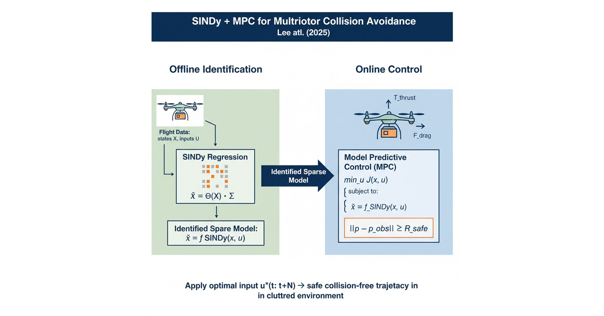
SINDy + MPC for Multirotor Collision Avoidance : When Data-Driven Identification Meets Predictive Control
A closer look at sparse dynamics identification and model predictive control for multirotor collision avoidance.
SINDy + MPC로 멀티로터 충돌 회피하기 : 데이터 기반 모델 식별이 만난 예측 제어
SINDy로 식별한 동역학 모델과 MPC를 결합해, 불확실한 멀티로터의 충돌 회피 문제를 푸는 과정을 살펴봅니다.
Contents
Paper: Lee et al., Sparse Identification of Nonlinear Dynamics‐Based Model Predictive Control for Multirotor Collision Avoidance, IET Control Theory & Applications, 2025. DOI: 10.1049/cth2.70049 · arXiv: 2412.06388
All figures in this post are reproduced directly from the paper above (with the author’s involvement).
Why this paper?
Strap a payload to a multirotor and the vehicle is no longer the one you modeled. Mass and inertia change, aerodynamic disturbances enter, and the controller starts to wobble. Now demand that the same vehicle track a reference trajectory while avoiding obstacles : and the problem becomes genuinely interesting.
This paper attacks the problem with a data-driven identification + model predictive control (MPC) combo. The identifier of choice is SINDy (Sparse Identification of Nonlinear Dynamics).
System model: a multirotor with payload
The 6-DOF dynamics considered in the paper are
\[\dot{\eta} = \nu, \qquad \dot{\nu} = \tfrac{1}{m_t}(R_{BI} f_t + f_a) - g\] \[\dot{\Omega} = R_\omega \omega, \qquad \dot{\omega} = I_t^{-1}\left(\tau_t + \tau_a - \omega \times I_t \omega \right)\]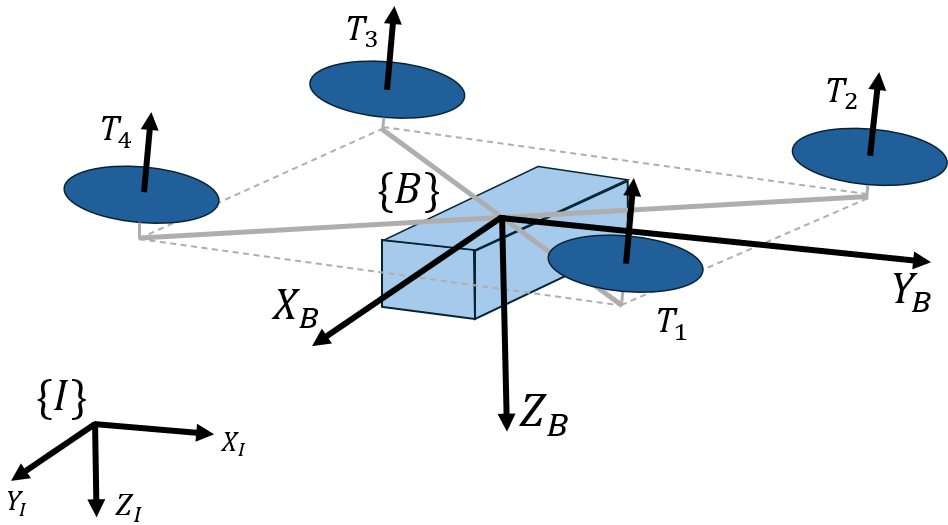 Fig. 1. Frame definitions for the payload-carrying multirotor: body frame ${B}$, inertial frame ${I}$, and rotor thrusts $T_1$-$T_4$. The payload changes both the mass and the inertia of the vehicle. (Source: Lee et al., 2025, Fig. 1)
The catch is that the payload changes mass and inertia:
- $m_t = m_m + m_p$
- $I_t = I_m + I_p$
Aerodynamic effects are modeled as linear damping:
- $f_a = [-K_F \dot{x},\ -K_F \dot{y},\ -K_F \dot{z}]^\top$
- $\tau_a = [-K_{M,p}\, p,\ -K_{M,q}\, q,\ -K_{M,r}\, r]^\top$
The practical issue is that $m_p$, $I_p$, $K_F$, and $K_M$ are all unknown. They must be estimated from data.
Why SINDy?
There is no shortage of ways to learn dynamics from data : neural networks, Gaussian processes, Koopman embeddings. They share one drawback: the resulting model is a black box. You cannot easily say which term in the dynamics caused a given output, nor can you give the model a physical meaning.
SINDy is different.
- It assumes that the governing equations of the system are sparse : only a small number of terms matter.
- A candidate function library $\Psi$ is regressed against state derivatives, and L1 regularization keeps only the meaningful coefficients.
- The result is a human-readable ODE that requires modest amounts of data.
For safety-critical aerospace applications, the interpretability of SINDy is a real asset.
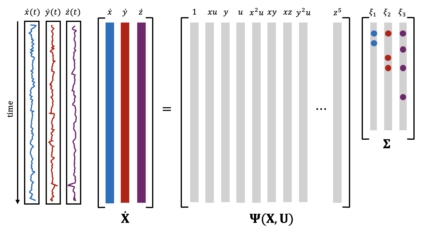 Fig. 2. The SINDy regression in pictures. From measured time signals $\dot x(t), \dot y(t), \dot z(t)$ we form $\dot X = \Psi(X,U)\Sigma$, where the library $\Psi$ holds candidate monomials and cross-products (e.g.\ $1, xu, y, x^2u, \ldots, z^5$) and the coefficient matrix $\Sigma$ is driven sparse by L1 regularization. (Source: Lee et al., 2025, Fig. 2)
SINDy in one equation
Stack the state snapshots into $X$ and their numerical derivatives into $\dot X$. Then regress
\[\dot X = \Psi(X,U)\, \Sigma\]with an L1 penalty on the coefficient matrix:
\[\Sigma^\star = \arg\min_\Sigma \, \| \dot X - \Psi(X,U)\Sigma \|_2^2 + \lambda \|\Sigma\|_1\]Larger $\lambda$ produces a sparser $\Sigma$, leaving only the dominant dynamics terms.
Embedding physical priors in the library
A clever element of the paper is that physics-informed terms are baked into the candidate library:
\[\Psi_{\text{tr}} = \big[\,\Psi_{\text{prior}}(\text{thrust, gravity}) \;\big|\; \Psi_{\text{poly}}(\text{velocity polynomials})\,\big]\] \[\Psi_{\text{ro}} = \big[\,\Psi_{\text{prior}}(\text{control, rotational coupling}) \;\big|\; \Psi_{\text{poly}}(\text{angular-rate polynomials})\,\big]\]This guides the regression toward physically plausible solutions even with limited data.
Where does the data come from?
Hovering yields almost no information. The authors instead fly a PID baseline controller along a rectangular reference trajectory for 100 s, logging states and inputs at $\Delta t = 0.002\,\text{s}$. Translation and rotation models are then identified separately.
SINDy-MPC: closing the loop with the identified model
The identified $\dot x = \hat f(x,u)$ is plugged directly into an MPC formulation:
\[\min_{u_1,\dots,u_N}\; \sum_{i=1}^{N} \big[\, (r_i - y_i)^\top Q (r_i - y_i) + u_i^\top R\, u_i \,\big]\]subject to
- $\dot x = \hat f(x,u)$ : SINDy-identified dynamics,
- $u_{\min} \le u \le u_{\max}$ : input bounds,
- $x_1 = x_{\text{init}}$ : initial state,
- $\sqrt{(x_{\text{ob}}-x)^2 + (y_{\text{ob}}-y)^2 + (z_{\text{ob}}-z)^2} \ge D_{\min}$ : collision avoidance.
The last constraint is what makes this work: a simple distance inequality forces the optimizer to bend the trajectory around obstacles.
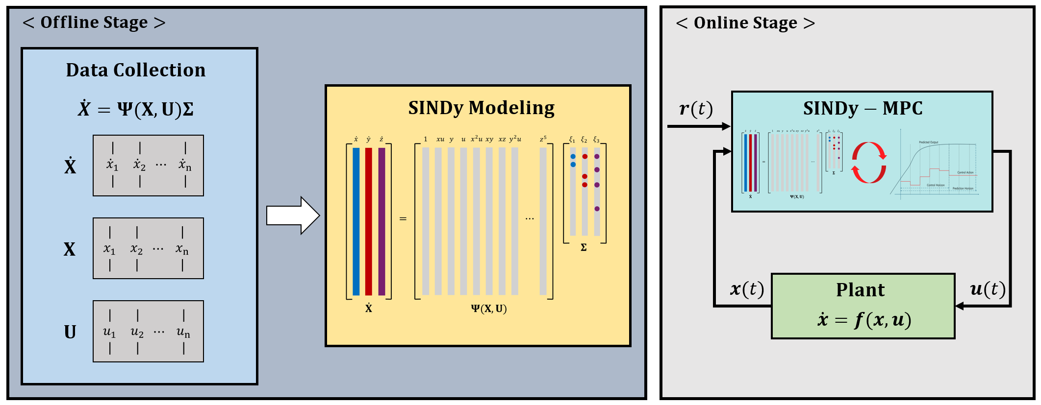 Fig. 3. The full SINDy-MPC pipeline. (Left) Offline stage : baseline-flight data $\dot X, X, U$ feeds a sparse regression that yields the library $\Psi(X,U)$ and a sparse $\Sigma$. (Right) Online stage : the identified model is plugged into an MPC that tracks $r(t)$ while closing the loop with the plant $\dot x = f(x,u)$. (Source: Lee et al., 2025, Fig. 3)
Identification accuracy (Tables II-III)
The paper reports true vs identified coefficients for the dominant terms of both translational and rotational dynamics. The key entries:
| Term | True $\Sigma$ | Identified $\hat\Sigma$ | Error |
|---|---|---|---|
| $R_{(1,3)} F_B \to \dot{x}$ | 0.7692 | 0.7707 | 0.20% |
| $R_{(2,3)} F_B \to \dot{y}$ | 0.7692 | 0.7704 | 0.16% |
| $L \to \dot{p}$ | 32.258 | 32.248 | 0.03% |
| $M \to \dot{q}$ | 26.316 | 26.316 | 0.00% |
| $N \to \dot{r}$ | 15.873 | 15.879 | 0.04% |
Every dominant coefficient is recovered to within 1%. The exception is yaw aerodynamic damping ($-K_{M,r} r$), where the rectangular reference simply does not excite yaw enough to identify the term reliably (>30% error). Excitation is part of the design problem.
Closed-loop performance (Table IV)
A direct comparison between the SINDy-MPC and the nominal-model MPC under the same payload + aerodynamic uncertainty:
| RMSE [m] | $x$ | $y$ | $z$ |
|---|---|---|---|
| SINDy-MPC | 0.813 | 0.381 | 0.399 |
| Nominal-model MPC | 0.909 | 0.452 | 0.628 |
The largest improvement is on the z axis (36% reduction, $0.628 \to 0.399$), which is exactly where unmodeled mass and aerodynamic drag hurt the most.
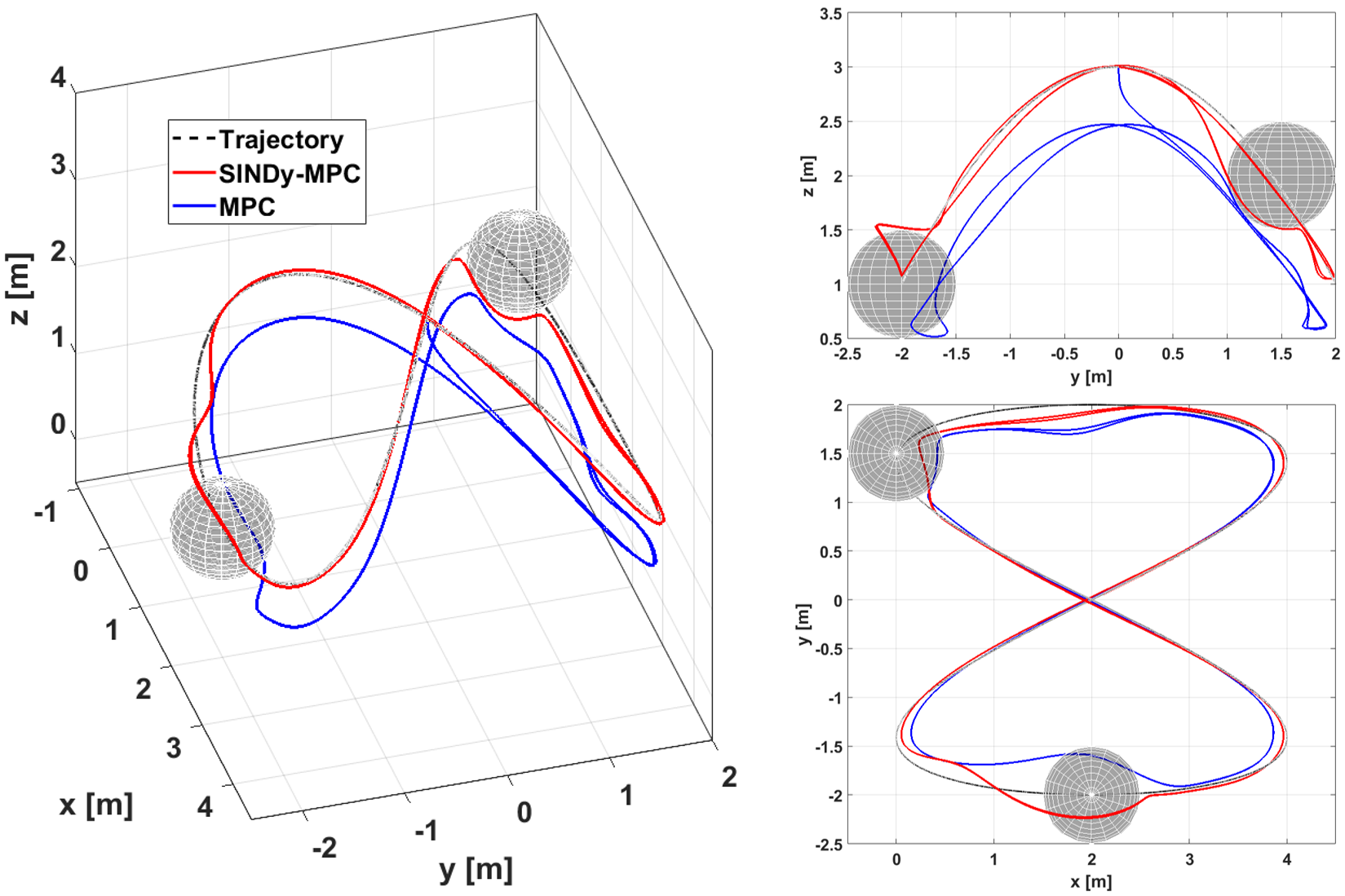 Fig. 4. 3D trajectory tracking. With a rectangular reference and two obstacles, SINDy-MPC follows the reference more closely while still keeping the safety distance from each obstacle. (Source: Lee et al., 2025, Fig. 8)
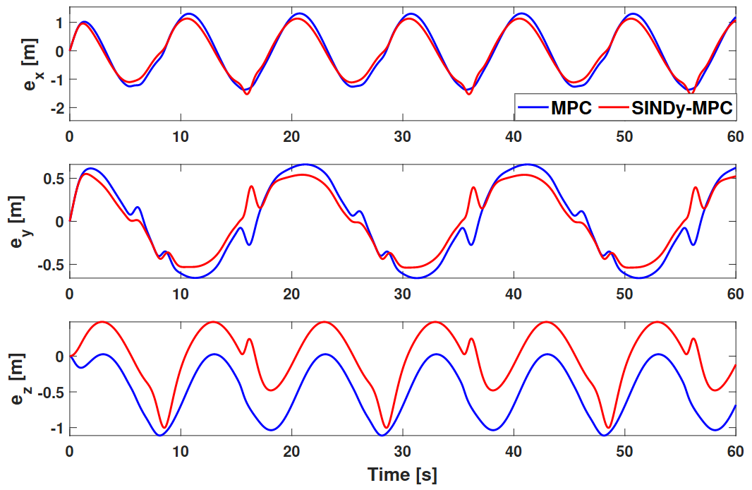 Fig. 5. Position-tracking error time histories. SINDy-MPC (blue) shows consistently smaller error than nominal-model MPC (red) on every axis, with the gap most pronounced on the z axis. (Source: Lee et al., 2025, Fig. 9)
Contributions in one paragraph
- A meaningful multirotor model that explicitly accounts for payload and aerodynamic uncertainty.
- The first SINDy + MPC framework specifically targeted at multirotor collision avoidance.
- Embedding physical priors in the candidate library to combine data efficiency with model interpretability.
My take
In a world increasingly dominated by neural identifiers, this paper is a reminder that sparsity and interpretability still matter : especially in aerospace, where being able to explain why a model produces a given output is half the value.
The honest limitations:
- The result depends heavily on the chosen library : domain knowledge is unavoidable.
- Data distribution matters; the yaw case shows what happens when it does not.
- Online re-identification and adaptive SINDy are natural follow-up directions.
A real-flight implementation, plus an adaptive SINDy variant for changing payloads, would be the obvious next step.
References
- Original (IET CTA): https://ietresearch.onlinelibrary.wiley.com/doi/10.1049/cth2.70049
- arXiv preprint: https://arxiv.org/abs/2412.06388
- Brunton, S. L., Proctor, J. L., & Kutz, J. N. (2016). Discovering governing equations from data by sparse identification of nonlinear dynamical systems. PNAS.
- Kaiser, E., Kutz, J. N., & Brunton, S. L. (2018). Sparse identification of nonlinear dynamics for model predictive control in the low-data limit. Proc. R. Soc. A.
Figure provenance
All figures in this post are reproduced directly from Lee et al. (2025) : the original paper of the post’s author. The original figure number from the paper is given in each caption.
Corrections welcome. As always, the paper itself is the best source.
Paper: Lee et al., Sparse Identification of Nonlinear Dynamics‐Based Model Predictive Control for Multirotor Collision Avoidance, IET Control Theory & Applications, 2025. DOI: 10.1049/cth2.70049 · arXiv: 2412.06388
본 글에 인용된 모든 그림은 위 논문(저자 본인 포함)에서 가져온 것입니다.
들어가며
드론(멀티로터)에 페이로드를 매달면 어떻게 될까요? 질량과 관성이 바뀌고, 공기역학적 외란까지 추가됩니다. 모델은 부정확해지고, 제어기는 갑자기 흔들리기 시작합니다. 이런 상황에서도 궤적을 따라가면서 동시에 장애물을 피해야 한다면, 어떻게 해야 할까요?
오늘 소개할 논문은 이 문제를 데이터 기반 시스템 식별 + 모델 예측 제어(MPC) 로 푸는 흥미로운 접근을 보여줍니다. 핵심은 SINDy(Sparse Identification of Nonlinear Dynamics) 입니다.
시스템 모델: 페이로드를 단 멀티로터
논문에서 다루는 6-DOF 동역학은 다음과 같습니다.
\[\dot{\eta} = \nu, \qquad \dot{\nu} = \tfrac{1}{m_t}(R_{BI} f_t + f_a) - g\] \[\dot{\Omega} = R_\omega \omega, \qquad \dot{\omega} = I_t^{-1}\left(\tau_t + \tau_a - \omega \times I_t \omega \right)\] 그림 1. 페이로드를 매단 멀티로터의 좌표계 정의. body frame ${B}$ 와 inertial frame ${I}$, 그리고 네 개의 로터 추력 $T_1$-$T_4$. 페이로드 박스가 추가되어 질량과 관성이 변한다. (출처: Lee et al., 2025, Fig. 1)
여기서 핵심은 페이로드 때문에 질량/관성이 바뀐다는 점입니다.
- $m_t = m_m + m_p$
- $I_t = I_m + I_p$
추가로 공기역학 효과를 선형 감쇠로 모델링합니다.
- $f_a = [-K_F \dot{x},\ -K_F \dot{y},\ -K_F \dot{z}]^\top$
- $\tau_a = [-K_{M,p}\, p,\ -K_{M,q}\, q,\ -K_{M,r}\, r]^\top$
문제는? $m_p, I_p, K_F, K_M$ 모두 정확히 모릅니다. 그래서 데이터로 알아내야 합니다.
왜 SINDy인가?
데이터로 모델을 학습하는 방법은 많습니다. 신경망(DNN), 가우시안 프로세스(GP) 등이 대표적이죠. 그런데 이 방법들은 모두 블랙박스입니다. 모델이 왜 그런 출력을 내는지, 물리적으로 어떤 의미인지 설명하기가 어렵습니다.
SINDy는 다릅니다.
- “시스템을 지배하는 방정식은 사실 몇 개의 항으로 충분히 표현된다”는 가정에서 출발합니다.
- 후보 함수 라이브러리 $\Psi$ 에서 희소(sparse) 계수만 골라내어, 사람이 읽을 수 있는 ODE 형태의 모델을 만듭니다.
- 적은 데이터로도 작동하고, 결과가 물리적으로 해석 가능합니다.
이 점이 안전이 중요한 멀티로터 제어에서 큰 장점이 됩니다.
그림 2. SINDy의 기본 아이디어. 시간에 따라 측정된 상태 시그널 $\dot x(t)$, $\dot y(t)$, $\dot z(t)$ 로부터 $\dot X = \Psi(X,U)\Sigma$ 의 회귀를 푼다. 라이브러리 $\Psi$ 는 후보 단항/곱셈 항(예: $1, xu, y, x^2u, \ldots, z^5$)으로 구성되며, 계수 행렬 $\Sigma$ 는 L1 정칙화에 의해 희소하게 만들어진다. (출처: Lee et al., 2025, Fig. 2)
SINDy의 핵심 식
상태 스냅샷 $X$ 와 그 미분 $\dot X$ 를 모은 뒤, 후보 함수 라이브러리 $\Psi(X,U)$ 로 회귀합니다.
\[\dot X = \Psi(X,U)\, \Sigma\]여기서 계수 $\Sigma$ 를 L1 정칙화로 희소하게 만듭니다.
\[\Sigma^\star = \arg\min_\Sigma \, \| \dot X - \Psi(X,U)\Sigma \|_2^2 + \lambda \|\Sigma\|_1\]$\lambda$ 가 클수록 거의 0인 항이 잘려나가고, 결국 진짜 의미 있는 항만 남습니다.
후보 라이브러리에 물리 지식 주입
논문이 영리한 점은 사전 지식을 라이브러리에 함께 넣어준다는 것입니다.
\[\Psi_{\text{tr}} = \big[\,\Psi_{\text{prior}}(\text{thrust, gravity}) \;\big|\; \Psi_{\text{poly}}(\text{velocity polynomials})\,\big]\] \[\Psi_{\text{ro}} = \big[\,\Psi_{\text{prior}}(\text{control, rotational coupling}) \;\big|\; \Psi_{\text{poly}}(\text{angular-rate polynomials})\,\big]\]이렇게 하면 데이터가 적어도 SINDy가 옳은 방향으로 빠르게 수렴합니다.
데이터를 어떻게 모았나?
가만히 호버링만 해서는 다양한 동역학을 관측할 수 없습니다. 그래서 베이스라인 PID 제어기로 사각형 궤적을 따라 100초간 비행하면서 $\Delta t = 0.002\,\text{s}$ 간격으로 데이터를 수집합니다. 이렇게 모은 데이터를 SINDy에 넣어 병진(translation) 과 회전(rotation) 모델을 따로 식별합니다.
SINDy-MPC: 식별된 모델로 제어하기
SINDy가 만든 모델 $\dot x = \hat f(x,u)$ 를 그대로 MPC에 꽂습니다.
\[\min_{u_1,\dots,u_N}\; \sum_{i=1}^{N} \big[\, (r_i - y_i)^\top Q (r_i - y_i) + u_i^\top R\, u_i \,\big]\]제약 조건:
- $\dot x = \hat f(x,u)$ : SINDy 모델
- $u_{\min} \le u \le u_{\max}$ : 제어 입력 한계
- $x_1 = x_{\text{init}}$ : 초기 상태
- $\sqrt{(x_{\text{ob}}-x)^2 + (y_{\text{ob}}-y)^2 + (z_{\text{ob}}-z)^2} \ge D_{\min}$ : 충돌 회피
마지막 제약이 핵심입니다. 장애물과의 거리를 부등식 제약으로 박아 넣어, MPC가 자연스럽게 회피 경로를 만들도록 합니다.
그림 3. SINDy-MPC 전체 흐름. (좌) Offline stage : 베이스라인 비행으로 모은 $\dot X$, $X$, $U$ 데이터로 라이브러리 $\Psi(X,U)$ 와 sparse $\Sigma$ 를 식별한다. (우) Online stage : 식별된 모델을 MPC에 그대로 넣고, 참조 $r(t)$ 를 추종하면서 plant $\dot x = f(x,u)$ 와 폐루프를 형성한다. (출처: Lee et al., 2025, Fig. 3)
결과: 식별 정확도 (논문 Table II-III)
논문은 병진/회전 모델 각각에 대해 dominant한 계수의 참값과 식별값을 제공합니다. 핵심 항만 추리면 다음과 같습니다.
| 계수 | 참값 ($\Sigma$) | 식별값 ($\hat\Sigma$) | 오차 |
|---|---|---|---|
| $R_{(1,3)} F_B \to \dot{x}$ | 0.7692 | 0.7707 | 0.20% |
| $R_{(2,3)} F_B \to \dot{y}$ | 0.7692 | 0.7704 | 0.16% |
| $L \to \dot{p}$ | 32.258 | 32.248 | 0.03% |
| $M \to \dot{q}$ | 26.316 | 26.316 | 0.00% |
| $N \to \dot{r}$ | 15.873 | 15.879 | 0.04% |
거의 모든 항이 1% 미만의 오차로 회복됩니다. 다만 yaw 공기역학($-K_{M,r} r$)은 사각형 궤적에 yaw 변화가 거의 없어서 30% 이상의 오차를 보였는데, 이는 데이터 수집 전략의 중요성을 잘 보여주는 부분이기도 합니다.
폐루프 제어 성능 (논문 Table IV)
페이로드/공기역학 효과를 모르는 nominal MPC와 SINDy-MPC를 같은 환경에서 비교한 결과:
| RMSE [m] | $x$ | $y$ | $z$ |
|---|---|---|---|
| SINDy-MPC | 0.813 | 0.381 | 0.399 |
| Nominal-model MPC | 0.909 | 0.452 | 0.628 |
특히 z축에서 36% 개선($0.628 \to 0.399$)이 나타납니다.
그림 4. 3D 궤적 추종 결과. 사각형 reference (점선)에 두 개의 장애물이 있는 환경에서, SINDy-MPC가 reference에 더 가깝게 따라가며 장애물을 회피하는 모습. (출처: Lee et al., 2025, Fig. 8)
그림 5. 위치 오차 시계열. 모든 축에서 SINDy-MPC(파랑)가 nominal-model MPC(빨강)보다 일관되게 작은 오차를 보인다. 특히 z축에서 차이가 두드러진다. (출처: Lee et al., 2025, Fig. 9)
이 논문의 기여를 정리하면
- 페이로드 + 공기역학 불확실성을 동시에 다루는 의미 있는 멀티로터 모델 식별
- SINDy + MPC를 멀티로터 충돌 회피에 결합한 최초의 시도
- 사전 물리 지식을 라이브러리에 결합해 데이터 효율 + 해석 가능성 동시 확보
개인적인 감상
신경망 기반 시스템 식별이 대세인 요즘, 희소성과 해석 가능성을 무기로 하는 SINDy의 부활을 보는 느낌입니다. 특히 안전 제약이 중요한 항공 분야에서는 “왜 이 모델이 이런 출력을 내는지”를 설명할 수 있다는 점이 큰 가치를 갖죠.
다만 한계도 분명합니다.
- 후보 라이브러리 설계가 결과를 크게 좌우 : 결국 사람의 도메인 지식이 필수
- 데이터 분포에 민감 (yaw 케이스가 그 예)
- 온라인 모델 업데이트 시 SINDy를 어떻게 빠르게 다시 풀 것인가도 과제
후속 연구로 실제 비행 실험과 온라인 적응형 SINDy가 자연스럽게 나올 만한 그림입니다.
References
- 원문 (IET CTA): https://ietresearch.onlinelibrary.wiley.com/doi/10.1049/cth2.70049
- arXiv 프리프린트: https://arxiv.org/abs/2412.06388
- Brunton, S. L., Proctor, J. L., & Kutz, J. N. (2016). Discovering governing equations from data by sparse identification of nonlinear dynamical systems. PNAS.
- Kaiser, E., Kutz, J. N., & Brunton, S. L. (2018). Sparse identification of nonlinear dynamics for model predictive control in the low-data limit. Proc. R. Soc. A.
그림 출처
본 글에 인용된 그림은 모두 Lee et al. (2025)의 figure를 그대로 가져온 것입니다 (저자 본인 포함). 각 그림 캡션에 원문에서의 figure 번호를 명시했습니다.
잘못된 부분이 있다면 알려주세요. 가능하면 논문을 직접 읽어보시길 추천드립니다.